M6 Surface Sensitivity
Deriving the surface sensitivity can be an incredibly useful tool in wing design toidentify the areas where drag reduction can be achieved. In this case, the flow condition is chosen as Mach=0.84, Re=11.72 x 10⁶ and Cl=0.2743. The mesh adjoint is first calculated for the original wing geometry. The wing surface points are only moving along the z-direction. Therefore, only λmesh,z (also referred to as lambda_gz) is used. λmesh,z are the sensitivities of Cd w.r.t. changes of the surface in the z-direction. The contour of λmesh,z is plotted in the following figure.
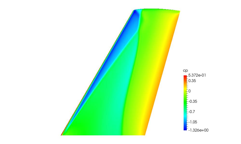
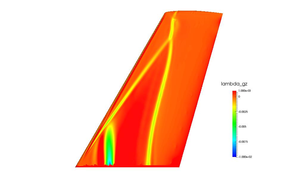
The figure on the right shows the negative surface sensitivity on the upper surface of the M6 wing. The green, blue and yellow areas on the surface in the figure on the right show regions where the gradient points in a positive z-direction. This implies that the drag reduces as the surface moves outwards (+z-direction). The red regions show areas with negative or very small derivatives. On the M6 wing the sensitivity makes a clear lambda structure. The pressure plot on the left confirms the lambda structure can be attributed to the shock locations. In addition to this there is a non-shock region near the wing root which suggests moving the surface in a positive z-direction in that region could also achieve a drag change. This is not shown in the surface pressure plot.
Previous research by Qin et al. has focussed on optimising a shock bump array on the rear shock line only (neglecting near the tip). This work takes this further by applying bumps over the entire span of the wing. Furthermore, it explores surface changes in the front shock region and the sensitive non-shock region near the wing root.
M6 3D bump array optimisation
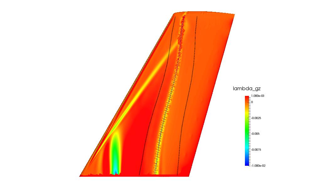
The surface mesh points with large negative λmesh values, shown in blue, green and yellow colour in the above figure. The rear shock line has the greatest potential for shock bump deployment as it shows the largest sensitivities of the two shock lines. First, the rear shock line is extracted then the points are fitted and smoothed using 5th order polynomials. The sensitivities feature line is then obtained for distributing the shock control bumps.
In order to achieve the best result from shock control, it is particularly important to involve the wing tip region where the sensitivity is strongest. The bump is deployed starting at y=0.01m and ending at y=1.19m. 14 bumps are evenly distributed, which gives a bump width of 0.084m. The optimisation region is defined by a front line and rear line, specifying the extension of the bumps. The distance between these lines is defined by xlength (y)=0.35 x Chordwing (y) based on our previous experience on shock control bump designs. This means that at any span position, the local length of the bump is equal to 35% wing local chord. This is based on previous research by Wong et al. and Qin et al., which suggested that the shock control bump length should be between 20% to 40% chord length. Finally, the bump has to be deployed w.r.t. the shock feature line. The previuos research [Qin et al.] and EUROSHOCK II project suggested that the peak of shock control bump should be between 5-10% downstream of the shock for an asymmetric bump. The bump will be placed downstream in terms of shock feature line. In this case, it has 40% length in front of shock feature line and 60% behind. The following figure shows the bounds of the optimisation region.
After the bump area is decided, the optimization can be carried out. In this case, the Bernstein polynomials for each bump have 3rd order chordwise, 3rd order spanwise, and 3rd order of the height distribution. The length and width of the bumps are fixed, hence the total number of design variables is [14×((4×4)+4)]=280.
During the flow calculation the lift is constrained to guarantee the target Cl is matched. The objective function is then modified as:
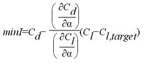
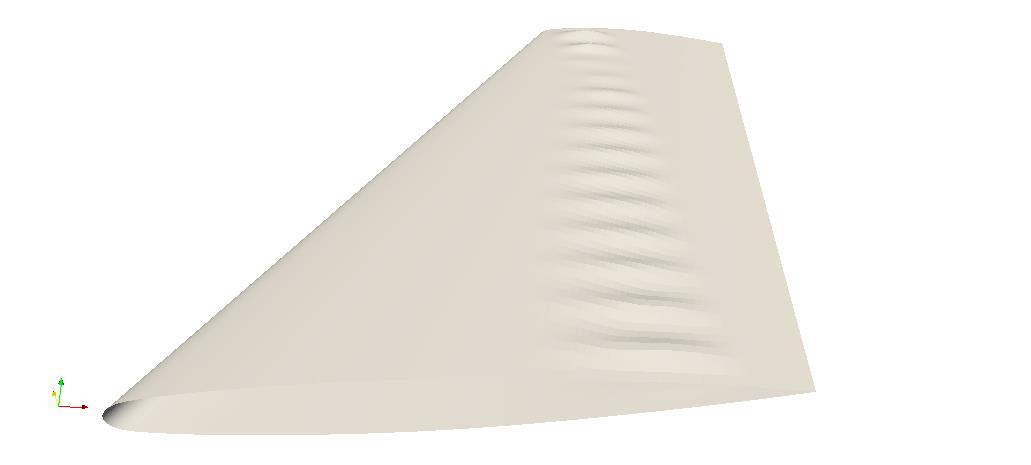
The following figure shows the topology of the bumps on the M6 wing for the final iteration in the optimisation. It is obvious that at the tip the bumps are the tallest. This is what we would expect since the sensitivities in the positive z-direction at this location are very strong. It is also interesting to note that at the region where the ‘legs’ of the LAMBDA-shock concatenate, the shock bump height is very close to zero. In this region the possible reduction of wave drag for one of the shocks is offset by an increase of drag elsewhere, therefore the optimiser has driven the bump height to be smaller in this region. The highest bumps are found at the tip region on the wing where the wave drag is largest. The wave drag has been reduced all across the span when bumps are present, however at the tip there is still a significant amount of wave drag generated which could be reduced further.

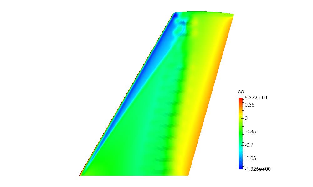
The following figures show the surface pressure distribution on the upper surface of the M6 wing. The wing with no bumps shows a very sharp change in pressure at the rear shock line which is smoothened in the case with the optimised bumps included. When the optimised bumps are placed on the wing the pressure change in the rear shock line region is much more gradual across the majority of the span. The pressure change has been reduced in most of the wing tip area but there is still a small region in between the bumps which contains a sharp change in pressure which is indicative of a small shock.
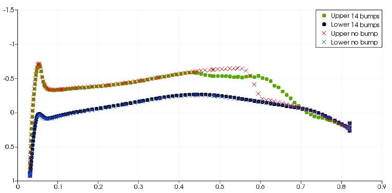
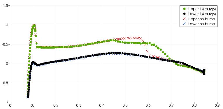
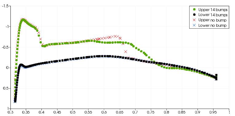
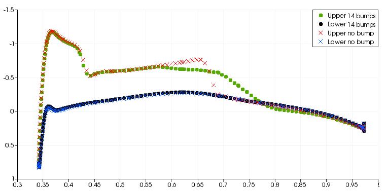
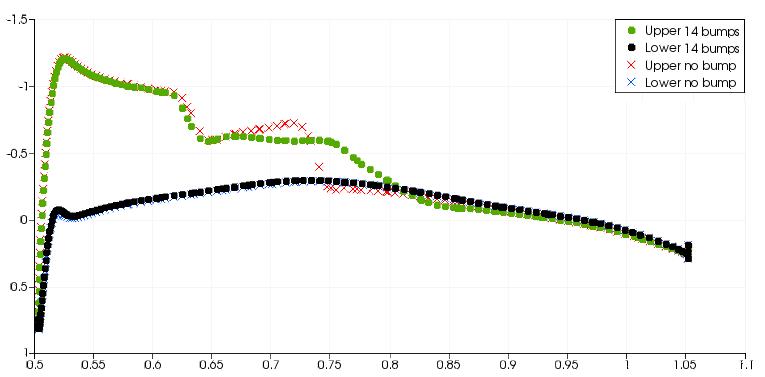
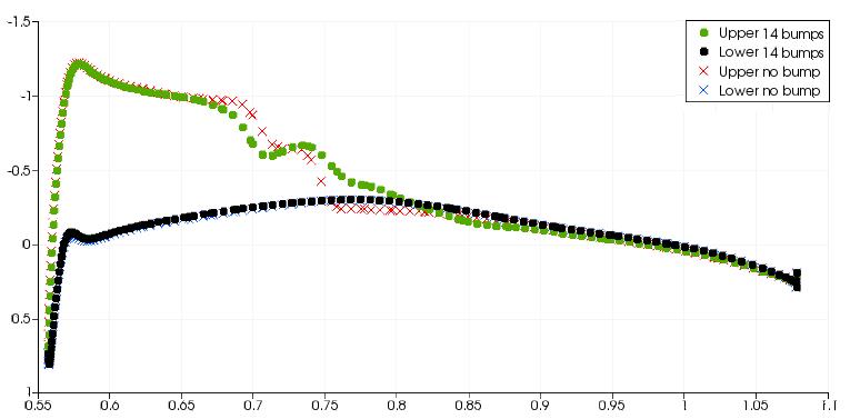
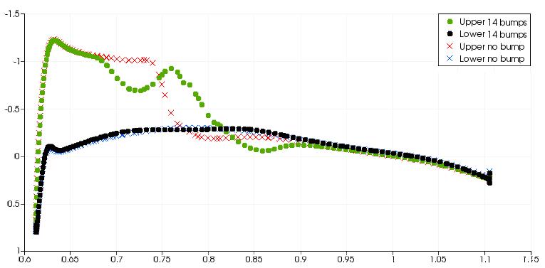
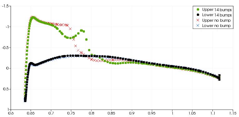
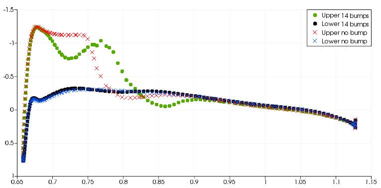
The above figure shows spanwise slices along the M6 wing and the surface pressure distribution is plotted on each slice. For the 1st through to 11th the bump, the pressure distribution at the rear shock shows a much more gradual change. This effect on the pressure distribution is typical of a well designed shock bump. The 12th bump is in the region where the front and rear shocks join. There is still a positive effect on the rear shock but it is much less significant in comparison to the bumps closer to the wing root. For bumps 13 and 14 at the wing tip, there is a strong reexpansion of the flow after the initial compression However the pressure change after the re-expansion is not as severe. Between the 13th and 14th bumps, there is a strong re-expansion of the flow and the gradient of pressure after the re-expansion is still large, indicative of a shock wave.